본 게시글에서는 머신러닝의 앙상블 모델인 Random Forest와 Gradient Boost 기법의 종류인 XGBoost와 LightGBM를 사용하여 예측을 진행한다. XGBoost와 LightGBM 기법은 최근 Kaggle 플랫폼에서 좋은 성능을 보이며 주목을 받고 있다. 하지만 두 모델 모두 의사결정나무 (Decision Tree)를 기반으로 하기 때문에 오버 피팅 (Over-fitting)에 주의해야 한다.
부스팅은 랜덤 포레스트나 배깅처럼 여러 개의 트리를 만드나 기존에 있는 예측기를 발전시켜서 이를 합한다는 차이점이 있다. 정리해보면 배깅은 모델을 다양하게 만들기 위해 데이터를 재구성하는 방법, 랜덤 포레스트는 모델을 다양하게 만들기 위해 데이터와 변수 모두 재구성하는 방법 그리고 부스팅은 맞추기 어려운 데이터에 대해 가중치를 두어 학습하는 개념이다. 부스팅 기법들 간 차이는 오분류된 데이터를 다음 단계에서 어떻게 반영할 것인가의 차이에 있다. 그라디언트 부스팅은 이전 단계 합성 분류기의 데이터의 오차를 예측하는 새로운 약한 분류기를 학습하는 기법이다.
XGBoost (eXtreme Gradient Boosting)
XGBoost Gradient 는 병렬 처리와 최적화를 장점으로 내세우는 Boositng 알고리즘으로 출시된 이래 Kaggle 등 각종 대회에서 좋은 성적을 보이며 많은 주목을 받는 방법이다. XGBoost는 CART(Classification And Regression Tree)를 기반으로 만들어진 알고리즘으로 의사결정나무 기반의 앙상블 모델이다. 앙상블 모델은 다수의 학습방법을 이용하여 결론을 내리는 방법으로 CART는 이 여러 가지 의사결정나무를 통한 방법론이다. [1]
LightGBM (Light Gradient Boosting Machine)
LightGBM은 XGBoost와 다르게 Leaf-wise loss 방식을 사용하여 손실 함수(loss function)를 더 줄일 수 있다. 다른 알고리즘들은 트리가 수평적으로 확장되는 반면 LightGBM은 트리가 수직적으로 확장된다. 동일한 가지를 확장 할 때, Leaf-wise 알고리즘은 Level-wise 알고리즘보다 더 많은 손실을 줄일 수 있다. 빅데이터 시대가 도래하면서 다루어야 하는 데이터의 크기와 규모는 점점 커지고 있으며 기존의 데이터 분석 알고리즘은 대규모의 데이터를 다루기에 속도가 느리다. 이를 보완하는 모델이 LightGBM이며 LightGBM은 크기가 큰 데이터를 다루면서 적은 메모리를 차지하고 빠른 처리속도를 가지고 있다. 또한, 결과의 정확도에 초점을 맞춘 알고리즘이라는 장점도 있다.
Random Forest
랜덤 포레스트는 의사결정나무의 단점인 큰 분산을 보완하기 위해 더 많은 무작위성을 주어 약한 학습기들을 만들고 이를 선형으로 결합하여 최종 학습기를 만드는 방법이다. 랜덤 포레스트는 이론적 설명, 최종 결과에 대한 해석이 어려우나 예측 면에 있어서는 정확도가 매우 높은 방법으로 알려져 있다. 랜덤 포레스트는 무작위성을 최대한으로 주기 위해 붓 스트랩과 더불어 입력 변수들에 대한 무작위 추출을 결합한다. 따라서 연관성이 약한 학습기를 여러 개 만드는 방법이라고 할 수 있다. 랜덤 포레스트는 배깅모델과 비슷하나 배깅은 모델을 다양화하기 위해 데이터를 재구성하는 방법이고, 랜덤 포레스트는 데이터뿐만 아니라 변수를 재구성한다. 이는 모델의 분산을 줄이고 일반적인 배깅의 성능보다 우수한 성능을 보이게 한다. 배깅은 전체 데이터 세트에서 복원 추출을 하였으나, 각각의 의사결정 나무들은 중복되는 데이터를 다수 가지고 있기 때문에 독립이라는 보장이 없다. 즉, 비슷한 트리가 만들어질 확률이 높기 때문에 공분산이 0이 될 수 없으며, 트리가 증가함에 따라 오히려 모델 전체의 분산이 증가할 수 도 있게 된다. 이러한 의사결정나무 간 공분산을 줄일 수 있는 방법이 필요하며 랜덤 포레스트를 통해 이를 공분산을 줄일 수 있다. 랜덤 포레스트는 데이터뿐만 아니라, 변수도 무작위로 뽑아서 다양한 모델을 만들며, 이는 기본 모델 간의 공분산을 줄일 수 있다. 모델의 분산을 줄일 수 있는 랜덤 포레스트는 일반적으로 배깅보다 성능이 우수하다.
1. Library Import
먼저 Boost model이 없는 경우 설치를 한다.
pip install xgboostpip install lightgbmimport pandas as pd
import numpy as np
from sklearn.preprocessing import LabelEncoder
import seaborn as sns
import warnings
import matplotlib.pyplot as plt
from sklearn.metrics import mean_absolute_error
from sklearn.metrics import mean_squared_error
import os
from sacred import Experiment
from sacred.observers import FileStorageObserver
from xgboost import XGBRegressor
from lightgbm import LGBMRegressor
from sklearn.ensemble import RandomForestRegressor
import json
plt.style.use('ggplot')
warnings.filterwarnings('ignore')
%config InlineBackend.figure_format = 'retina'
PROJECT_ID='manifest-module-318307'
2. Sacred Setting
ex = Experiment('nyc-demand-prediction', interactive=True)

# experiment_dir가 없으면 폴더 생성하고 FileStorageObserver로 저장
experiment_dir = os.path.join('./', 'experiments')
if not os.path.isdir(experiment_dir):
    os.makedirs(experiment_dir)
ex.observers.append(FileStorageObserver.create(experiment_dir))
3. Data Pre-processing
%%time
base_query = """
WITH base_data AS
(
  SELECT nyc_taxi.*, gis.* EXCEPT (zip_code_geom)
  FROM (
    SELECT *
    FROM `bigquery-public-data.new_york_taxi_trips.tlc_yellow_trips_2015`
    WHERE
        EXTRACT(MONTH from pickup_datetime) = 1
        and pickup_latitude  <= 90 and pickup_latitude >= -90
    ) AS nyc_taxi
  JOIN (
    SELECT zip_code, state_code, state_name, city, county, zip_code_geom
    FROM `bigquery-public-data.geo_us_boundaries.zip_codes`
    WHERE state_code='NY'
    ) AS gis
  ON ST_CONTAINS(zip_code_geom, st_geogpoint(pickup_longitude, pickup_latitude))
)

SELECT
    zip_code,
    DATETIME_TRUNC(pickup_datetime, hour) as pickup_hour,
    EXTRACT(MONTH FROM pickup_datetime) AS month,
    EXTRACT(DAY FROM pickup_datetime) AS day,
    CAST(format_datetime('%u', pickup_datetime) AS INT64) -1 AS weekday,
    EXTRACT(HOUR FROM pickup_datetime) AS hour,
    CASE WHEN CAST(FORMAT_DATETIME('%u', pickup_datetime) AS INT64) IN (6, 7) THEN 1 ELSE 0 END AS is_weekend,
    COUNT(*) AS cnt
FROM base_data
GROUP BY zip_code, pickup_hour, month, day, weekday, hour, is_weekend
ORDER BY pickup_hour
"""

base_df = pd.read_gbq(query=base_query, dialect='standard', project_id='manifest-module-318307')
이번에는 Linear Regression과 다르게 One Hot Encoding이 아닌 Label Encoding을 사용한다.
One Hot Encoding과 Label Encoding은 데이터에 따라 어떤 방식이 좋은지 다르니, 두가지를 모두 사용해보고 어떤 방식을 사용할지 결정하는 것이 좋다.
le = LabelEncoder()
base_df['zip_code_le'] = le.fit_transform(base_df['zip_code'])
def split_train_and_test(df, date):
"""
Dataframe에서 train_df, test_df로 나눠주는 함수
df : 시계열 데이터 프레임
date : 기준점 날짜
"""
train_df = df[df['pickup_hour'] < date]
test_df = df[df['pickup_hour'] >= date]
return train_df, test_df
4. Train and Test Data Split
train_df, test_df = split_train_and_test(base_df, '2015-01-24')del train_df['zip_code']
del train_df['pickup_hour']
del test_df['zip_code']
del test_df['pickup_hour']y_train_raw = train_df.pop('cnt')
y_test_raw = test_df.pop('cnt')x_train = train_df.copy()
x_test = test_df.copy()
5. Modeling and Evaluation
5-1 XGBoost
def evaluation(y_true, y_pred):
    y_true, y_pred = np.array(y_true), np.array(y_pred)
    mape = np.mean(np.abs((y_true - y_pred) / y_true)) * 100
    mae = mean_absolute_error(y_true, y_pred)
    mse = mean_squared_error(y_true, y_pred)
    score = pd.DataFrame([mape, mae, mse], index=['mape', 'mae', 'mse'], columns=['score']).T
    return score
@ex.config
def config():
max_depth=5
learning_rate=0.1
n_estimators=100
n_jobs=-1max_depth, learning_rate, n_estimators, n_jobs는 XGBoost의 하이퍼 파리미터(Hyper Parameter)들이다.
모델이 데이터를 통해 학습하면서 성능을 높이기 위해 모델 내부에서 자체적으로 결정되는 매개변수인 파라미터와 달리, 하이퍼 파라미터는 초매개변수로써, 모델을 만들 때 사용자가 직접 설정하는 값이다. 하이퍼 파라미터는 모델의 성능에 큰 영향을 주지만, 학습을 하면서 스스로 찾는 값은 아니기 때문에 사용자가 여러 값들을 직접 수정해가면서 최적의 값을 찾아가야 한다.
@ex.capture
def get_model(max_depth, learning_rate, n_estimators, n_jobs):
    return XGBRegressor(max_depth=max_depth, learning_rate=learning_rate, n_estimators=n_estimators, n_jobs=n_jobs)
@ex.main
def run(_log, _run):
global xgb_reg, xgb_pred
xgb_reg = get_model()
xgb_reg.fit(x_train, y_train_raw)
xgb_pred = xgb_reg.predict(x_test)
score = evaluation(y_test_raw, xgb_pred)
_run.log_scalar('model_name', xgb_reg.__class__.__name__)
_run.log_scalar('metrics', score)
return score.to_dict()experiment_result = ex.run()
experiment_result.configfrom io import StringIO
def parsing_output(ex_id):
with open(f'./experiments/{ex_id}/metrics.json') as json_file:
json_data = json.load(json_file)
with open(f'./experiments/{ex_id}/config.json') as config_file:
config_data = json.load(config_file)
output_df = pd.DataFrame(json_data['model_name']['values'], columns=['model_name'], index=['score'])
output_df['experiment_num'] = ex_id
output_df['config'] = str(config_data)
values_data = StringIO(json_data['metrics']['values'][0]['values'])
metric_df = pd.read_csv(values_data)
output_df = pd.concat([output_df.reset_index(drop=True),
metric_df.reset_index(drop=True)], axis=1)
return output_dfparsing_output(7)output(7)의 경우 위의 코드 실행중 몇 번의 오류가 있어 7번까지 실행이 되었다. 이 숫자는 experiment_result = ex.run()을 실행시킨 결과 값을 참고하면 된다. (Started run with ID "7)

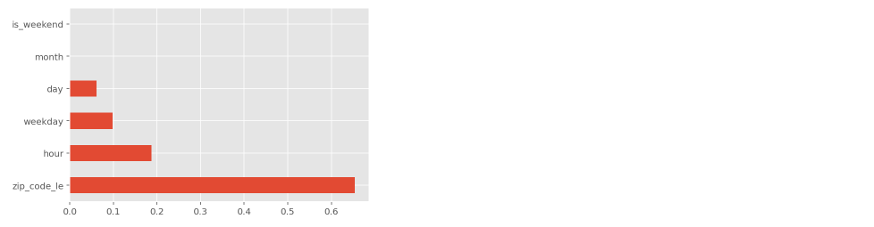
feat_importances = pd.Series(xgb_reg.feature_importances_, index=x_train.columns)
feat_importances.nlargest(15).plot(kind='barh')
추가로 결과에 대해 Feature importance를 확인해보면, zip code가 가장 큰 영향을 미치는 것을 볼 수 있으며 이후 hour, weekday, day 순인 것을 확인할 수 있다.
5-2 LightGBM
모델링 전단계까지는 모두 같은 절차이다.
@ex.config
def config():
    num_leaves=31
    max_depth=-1
    learning_rate=0.1
    n_estimators=100
@ex.capture
def get_model(num_leaves, max_depth, learning_rate, n_estimators):
return LGBMRegressor(num_leaves=num_leaves, max_depth=max_depth, learning_rate=learning_rate, n_estimators=n_estimators)@ex.main
def run(_log, _run):
global lgbm_reg, lgbm_pred
lgbm_reg = get_model()
lgbm_reg.fit(x_train, y_train_raw)
lgbm_pred = lgbm_reg.predict(x_test)
score = evaluation(y_test_raw, lgbm_pred)
_run.log_scalar('model_name', lgbm_reg.__class__.__name__)
_run.log_scalar('metrics', score)
return score.to_dict()experiment_result = ex.run()experiment_result.configdef parsing_output(ex_id):
with open(f'./experiments/{ex_id}/metrics.json') as json_file:
json_data = json.load(json_file)
with open(f'./experiments/{ex_id}/config.json') as config_file:
config_data = json.load(config_file)
output_df = pd.DataFrame(json_data['model_name']['values'], columns=['model_name'], index=['score'])
output_df['experiment_num'] = ex_id
output_df['config'] = str(config_data)
values_data = StringIO(json_data['metrics']['values'][0]['values'])
metric_df = pd.read_csv(values_data)
output_df = pd.concat([output_df.reset_index(drop=True),
metric_df.reset_index(drop=True)], axis=1)
return output_dfparsing_output(8)
feat_importances = pd.Series(lgbm_reg.feature_importances_, index=x_train.columns)
feat_importances.nlargest(15).plot(kind='barh')
5-3 Random Forest
@ex.config
def config():
n_estimators=10
n_jobs=-1@ex.capture
def get_model(n_estimators, n_jobs):
return RandomForestRegressor(n_estimators=n_estimators, n_jobs=n_jobs)@ex.main
def run(_log, _run):
global rf_reg, rf_pred
rf_reg = get_model()
rf_reg.fit(x_train, y_train_raw)
rf_pred = rf_reg.predict(x_test)
score = evaluation(y_test_raw, rf_pred)
_run.log_scalar('model_name', rf_reg.__class__.__name__)
_run.log_scalar('metrics', score)
return score.to_dict()experiment_result = ex.run()from io import StringIO
def parsing_output(ex_id):
    with open(f'./experiments/{ex_id}/metrics.json') as json_file:
        json_data = json.load(json_file)
    with open(f'./experiments/{ex_id}/config.json') as config_file:
        config_data = json.load(config_file)

    output_df = pd.DataFrame(json_data['model_name']['values'], columns=['model_name'], index=['score'])
    output_df['experiment_num'] = ex_id
    output_df['config'] = str(config_data)
    values_data = StringIO(json_data['metrics']['values'][0]['values'])
    metric_df = pd.read_csv(values_data)

    output_df = pd.concat([output_df.reset_index(drop=True),
                            metric_df.reset_index(drop=True)], axis=1)
return output_dfparsing_output(10)
feat_importances = pd.Series(rf_reg .feature_importances_, index=x_train.columns)
feat_importances.nlargest(15).plot(kind='barh')
다음 게시글에서는 3개 모델을 통해 예측한 결과에 대해 분석해야겠다.
'Programming > Project' 카테고리의 다른 글
| [NYC 택시 수요 예측 PJT] 10. Result Analysis and Feature Analysis (0) | 2021.08.19 |
|---|---|
| [NYC 택시 수요 예측 PJT] 8. 베이스라인 모델 구축 - 반복 실험(Sacred 사용) (0) | 2021.08.02 |
| [NYC 택시 수요 예측 PJT] 7. 베이스라인 모델 구축 (0) | 2021.07.28 |
| [NYC 택시 수요 예측 PJT] 6. 데이터 전처리 (2) | 2021.07.27 |
| [NYC 택시 수요 예측 PJT] 4. 데이터 EDA - 데이터 시각화 (Time Domain) - 2 (0) | 2021.07.14 |


