머신러닝 모델링을 진행하면 최적의 결과를 찾기 위해 다양한 모델을 사용하며 반복적으로 실험을 하게 된다. 이 과정에서 다양한 실험을 진행하며, feature, parameter를 자동으로 기록할 수 있는 도구가 있으면 진행이 아주 효율적인데 이때 Sacred라는 것을 사용하면 모델링을 할 때 사용했던 feature, parameter와 같은 설정을 저장하고 관리할 수 있다.
Scared Github에 의하면 Sacred는 실험에서 축적된 데이터의 복사를 만들고, 기록하고, 정리하고, 설정하는 데 도움을 주는 도구이며, 아래와 같이 설명하고 있다.
Sacred is a tool to help you configure, organize, log and reproduce experiments. It is designed to do all the tedious overhead work that you need to do around your actual experiment in order to:
- keep track of all the parameters of your experiment
- easily run your experiment for different settings
- save configurations for individual runs in a database
- reproduce your results
https://github.com/IDSIA/sacred
GitHub - IDSIA/sacred: Sacred is a tool to help you configure, organize, log and reproduce experiments developed at IDSIA.
Sacred is a tool to help you configure, organize, log and reproduce experiments developed at IDSIA. - GitHub - IDSIA/sacred: Sacred is a tool to help you configure, organize, log and reproduce expe...
github.com
Scared의 Main mechnisms의 아래와 같다.
- ConfigScopes : 함수의 local 변수를 편리하게 다룰 수 있고, @ex.config 데코레이터로 사용
- Config Injection : 모든 함수에 있는 설정을 접근할 수 있음
- Command-line interface : 커맨드 라인으로 parameter를 바꿔서 실행할 수 있음
- Observers : 실험의 모든 정보를 Observers에게 제공해 저장. MongoDB / S3 / Local에 저장 가능
- Automatic seeding : 실험의 무작위를 컨트롤할 때 도와줌
1. Sacred Install
!pip3 install sacred2. Library Import
import pandas as pd
from sklearn.preprocessing import OneHotEncoder, LabelEncoder
from sklearn.linear_model import LinearRegression
import seaborn as sns
import warnings
import matplotlib.pyplot as plt
from ipywidgets import interact
from sklearn.metrics import mean_absolute_error
from sklearn.metrics import mean_squared_error
import os
from numpy.random import permutation
from sklearn import datasets
from sacred import Experiment
from sacred.observers import FileStorageObserver

plt.style.use('ggplot')
warnings.filterwarnings('ignore')
%config InlineBackend.figure_format = 'retina'

PROJECT_ID='manifest-module-318307'
3. Data Pre-processing
ex = Experiment('nyc-demand-prediction', interactive=True)
# experiment_dir가 없으면 폴더 생성하고 FileStorageObserver로 저장
experiment_dir = os.path.join('./', 'experiments')
if not os.path.isdir(experiment_dir):
os.makedirs(experiment_dir)
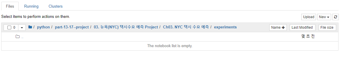
ex.observers.append(FileStorageObserver.create(experiment_dir))데이터 전처리를 하기 전 Sacred를 사용하기 위한 storage 폴더를 생성하고 데이터를 통합한다. 만약 폴더가 없다면 현재 경로에 'experiments'라는 폴더를 만들도록 한다. 실행하면 아래와 같이 experiments라는 폴더가 생성된다.
%%time
base_query = """
WITH base_data AS
(
  SELECT nyc_taxi.*, gis.* EXCEPT (zip_code_geom)
  FROM (
    SELECT *
    FROM `bigquery-public-data.new_york_taxi_trips.tlc_yellow_trips_2015`
    WHERE
        EXTRACT(MONTH from pickup_datetime) = 1
        and pickup_latitude  <= 90 and pickup_latitude >= -90
    ) AS nyc_taxi
  JOIN (
    SELECT zip_code, state_code, state_name, city, county, zip_code_geom
    FROM `bigquery-public-data.geo_us_boundaries.zip_codes`
    WHERE state_code='NY'
    ) AS gis
  ON ST_CONTAINS(zip_code_geom, st_geogpoint(pickup_longitude, pickup_latitude))
)

SELECT
    zip_code,
    DATETIME_TRUNC(pickup_datetime, hour) as pickup_hour,
    EXTRACT(MONTH FROM pickup_datetime) AS month,
    EXTRACT(DAY FROM pickup_datetime) AS day,
    CAST(format_datetime('%u', pickup_datetime) AS INT64) -1 AS weekday,
    EXTRACT(HOUR FROM pickup_datetime) AS hour,
    CASE WHEN CAST(FORMAT_DATETIME('%u', pickup_datetime) AS INT64) IN (6, 7) THEN 1 ELSE 0 END AS is_weekend,
    COUNT(*) AS cnt
FROM base_data
GROUP BY zip_code, pickup_hour, month, day, weekday, hour, is_weekend
ORDER BY pickup_hour
"""

base_df = pd.read_gbq(query=base_query, dialect='standard', project_id='manifest-module-318307')
4. Feature Engineering
enc = OneHotEncoder(handle_unknown='ignore')
enc.fit(base_df[['zip_code']])
ohe_output = enc.transform(base_df[['zip_code']]).toarray()
ohe_df = pd.concat([base_df, pd.DataFrame(ohe_output, columns='zip_code_'+enc.categories_[0])], axis=1)
ohe_df['log_cnt'] = np.log10(ohe_df['cnt'])
Feature engineer은 One Hot Encoding을 사용했던 지난 게시글에서 작성한 내용을 그대로 가져왔다.
https://sunghyeon.tistory.com/11
[NYC 택시 수요 예측 PJT] 7. 베이스라인 모델 구축
본 장에서는 수요 예측을 진행함에 있어 성능 비교의 기준이 되는 베이스라인 모델을 구축하고자 한다. 1. Library Import import pandas as pd from sklearn.preprocessing import OneHotEncoder from sklearn.li..
sunghyeon.tistory.com
5. Train Test Data Split
def split_train_and_test(df, date):
    """
    Dataframe에서 train_df, test_df로 나눠주는 함수

    df : 시계열 데이터 프레임
    date : 기준점 날짜
    """
    train_df = df[df['pickup_hour'] < date]
    test_df = df[df['pickup_hour'] >= date]
    return train_df, test_df
train_df, test_df = split_train_and_test(ohe_df, '2015-01-24')train_df.tail()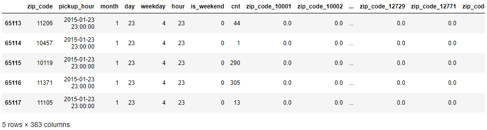
2015년을 1월 24일을 기준으로 train data와 test data를 나눴으므로 train data의 마지막 날짜와 시간을 보면 1월 23일 23시임을 확인할 수 있다.
# 사용하지 않을 column 삭제
del train_df['zip_code']
del train_df['pickup_hour']
del test_df['zip_code']
del test_df['pickup_hour']
y_train_raw = train_df.pop('cnt')
y_train_log = train_df.pop('log_cnt')
y_test_raw = test_df.pop('cnt')
y_test_log = test_df.pop('log_cnt')y_true = y_test_raw.values.copy()x_train = train_df.copy()
x_test = test_df.copy()
6. Evaluation
import numpy as np

def evaluation(y_true, y_pred):
    y_true, y_pred = np.array(y_true), np.array(y_pred)
    mape = np.mean(np.abs((y_true - y_pred) / y_true)) * 100
    mae = mean_absolute_error(y_true, y_pred)
    mse = mean_squared_error(y_true, y_pred)
    score = pd.DataFrame([mape, mae, mse], index=['mape', 'mae', 'mse'], columns=['score']).T
    return score
7. Experiment Setting
이 부분부터 본격적으로 Sacred와 NYC taxi data를 합친 것이며, 실험에 대한 셋팅을 설정한다.
7-1) Experiment Setting
@ex.config
def config():
    fit_intercept=True
    normalize=False
위에서 ex = Experiment('nyc-demand-prediction', interactive=True)를 했으며 본 데이터를 통한 실험에 대해 ex.config로 설정을 저장한다. config에 fit_intercept, normalize값을 넣어주며 fit_intercept, normalize는 dafulat값이다.
@ex.capture
def get_model(fit_intercept, normalize):
    return LinearRegression(fit_intercept, normalize)
ex.capture는 해당 설정을 사용해 함수를 리턴한다. 아래 코드의 run 아래 부분에 만들어도 되지만 따로 관리하기 위해 get_model 부분을 따로 만들었다.
# _log과 _run은 별도로 정의하지 않아도 함수의 인자로 사용 가능
@ex.main
def run(_log, _run):
    lr_reg = get_model() # get_model에 인자가 따로 안들어감 config에 있는 인자가 들어감
    lr_reg.fit(x_train, y_train_raw)
    pred = lr_reg.predict(x_test)
    # log File에 로그 저장
    _log.info("Predict End")
    score = evaluation(y_test_raw, pred)
    _run.log_scalar('model_name', lr_reg.__class__.__name__)

    # Metrics쪽에 저장하고 싶으면 아래처럼 사용
    _run.log_scalar('metrics', score)

    # Result쪽에 저장하고 싶으면 아래처럼 사용
    return score.to_dict()
experiment_result = ex.run()
위의 명령을 실행하면 experiments 폴더에 첫번째 실험인 1 폴더가 생성되고 그 안에 config, metric등 함수에 대한 설정이 기록으로 남게 된다.

experiment_result.config
7-2) Parser to verify experiment
experiment에서 log를 찍는 방식에 따라 사용하는 함수는 달라진다. 먼저 _run.log_scalar에 metrics를 저장하는 방법이 있고, @ex.main의 함수의 결과를 return하는 방법이 있다. 두 방법 중에는 _run.log_scalar에 metrics를 추천한다고 한다.
7-2-1) save metrics in _run.log_scalar
# 1) _run.log_scalar에 metrics을 저장하는 경우
def parsing_output(ex_id):
    with open(f'./experiments/{ex_id}/metrics.json') as json_file:
        json_data = json.load(json_file)
    with open(f'./experiments/{ex_id}/config.json') as config_file:
        config_data = json.load(config_file)

    output_df = pd.DataFrame(json_data['model_name']['values'], columns=['model_name'], index=['score'])
    output_df['experiment_num'] = ex_id
    output_df['config'] = str(config_data)
    metric_df = pd.DataFrame(json_data['metrics']['values'][0]['values'])

    output_df = pd.concat([output_df, metric_df], axis=1)
    output_df = output_df.round(2)
    return output_df
7-2-2) return output of @ex.main function
# 2) @ex.main의 함수에 결과를 return하는 경우
def parsing_output(ex_id):
    with open(f'./experiments/{ex_id}/run.json') as json_file:
        json_data = json.load(json_file)
    output = pd.DataFrame(json_data['result'])
return outputparsing_output(1)본 과정에서 error가 나왔는데 먼저 'name 'json' is not defined'라는 에러가 나왔으며 이는 import json을 통해 해결이 되었다. 이 과정에서 7-2-2)는 실행이 되나, 7-2-1)를 통한 함수는 output이 안나오는 것을 확인하였다.
7-2-1) 함수 실행후 parsing_output(1)을 실행하면 아래와 같은 에러가 나온다.
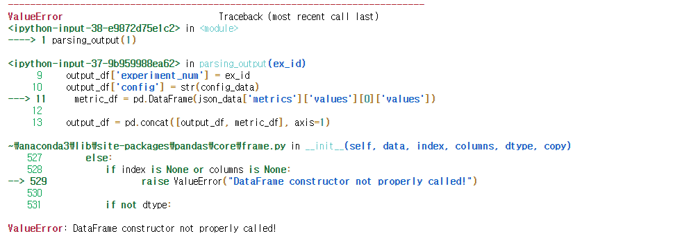
이 에러에 대해 찾아보니 DataFrame 형태가 list 형태로 되어있지 않기 때문이라고 한다. 그래서 DataFrame을 list형태로 바꾸어서 실행해보았다.
# 1) _run.log_scalar에 metrics을 저장하는 경우
def parsing_output(ex_id):
    with open(f'./experiments/{ex_id}/metrics.json') as json_file:
        json_data = json.load(json_file)
    with open(f'./experiments/{ex_id}/config.json') as config_file:
        config_data = json.load(config_file)

    output_df = pd.DataFrame(list(json_data['model_name']['values']), columns=['model_name'], index=['score'])
    output_df['experiment_num'] = ex_id
    output_df['config'] = str(config_data)
    metric_df = pd.DataFrame(list(json_data['metrics']['values'][0]['values']))

    output_df = pd.concat([output_df, metric_df], axis=1)
    output_df = output_df.round(2)
    return output_df
일단 실행은 되는데 이상한 결과가 나온다. 예상 결과는 model_name, experiemtn_num, config, mae, mape, mse 열을 가진 하나의 행의 결과가 나와야하는데 아직 문제가 있다.
내일 출근해야하니 퇴근하고 원인을 다시 찾아봐야겠다. 일단 잔다.
2021 08 02
어제 에러가 났던 부분에 대해 구글링을 해서 코드를 수정하고 결과를 뽑아냈다.
from io import StringIO

# 1) _run.log_scalar에 metrics을 저장하는 경우
def parsing_output(ex_id):
    with open(f'./experiments/{ex_id}/metrics.json') as json_file:
        json_data = json.load(json_file)
    with open(f'./experiments/{ex_id}/config.json') as config_file:
        config_data = json.load(config_file)

    output_df = pd.DataFrame(json_data['model_name']['values'], columns=['model_name'], index=['score'])
    output_df['experiment_num'] = ex_id
    output_df['config'] = str(config_data)
    values_data = StringIO(json_data['metrics']['values'][0]['values'])
    metric_df = pd.read_csv(values_data)

    output_df = pd.concat([output_df.reset_index(drop=True),
                            metric_df.reset_index(drop=True)], axis=1)
    output_df = output_df.round(3)
    return output_df
parsing_output(3)
처음부터 코드를 실행하여 세번째 실험이 되었고 이번에는 아웃풋이 제대로 나왔다.
'Programming > Project' 카테고리의 다른 글
| [NYC 택시 수요 예측 PJT] 10. Result Analysis and Feature Analysis (0) | 2021.08.19 |
|---|---|
| [NYC 택시 수요 예측 PJT] 9. XGBoost Regressor, LightGBM Regressor, Random Forest (0) | 2021.08.15 |
| [NYC 택시 수요 예측 PJT] 7. 베이스라인 모델 구축 (0) | 2021.07.28 |
| [NYC 택시 수요 예측 PJT] 6. 데이터 전처리 (2) | 2021.07.27 |
| [NYC 택시 수요 예측 PJT] 4. 데이터 EDA - 데이터 시각화 (Time Domain) - 2 (0) | 2021.07.14 |


